The Implementation of a Contour Module for Music21
Marcos da Silva Sampaio – [email protected]
Universidade Federal da Bahia
Pedro Kroger – [email protected]
Universidade Federal da Bahia
Mara Pinheiro Menezes – [email protected]
Universidade Federal da Bahia
Jean Menezes da Rocha – [email protected]
Universidade Federal da Bahia
Natanael Ourives – [email protected]
Universidade Federal da Bahia
Dennis Queiroz de Carvalho – [email protected]
Universidade Federal da Bahia
In this paper we present a contour module for the Music21 toolkit. The theory of musical contour has operations such as similarly, matrices and reduction that have been used to analyze music from many composers. The contour module can calculate these operations quickly and since the Music21 toolkit reads files in the Humdrum and MusicXML formats, a large corpus of music is available for analysis. To the best of our knowledge, this is the only tool for contour processing available today.
We introduce some background information about the Contour Theory, how the contour module can be used and some contour analysis using Bach’s 371 Chorales.
1. Introduction
Contour is the shape or format of an object. Contours can be bi- or multidimensional, and can relate height to length or time. In music, contours can be abstracted from elements such as pitch, chord density, duration, timbre, and intensity. Melodic contours, for instance, are abstractions of pitches in time. Musical contour is an ordered set of elements, disregarding absolute values, enumerated with integers from 0 to n-1 where n is the contour cardinality [10]. The study of contour is important because they can contribute to musical coherence (similarly to motifs and pitch class sets).
The theory of musical contour provides many operations such as vectors and arrays (Friedmann 1985), similarity (Marvin 1988), fuzzy similarity (Quinn 1997), matrices (Morris 1993), (Quinn 1997) and reduction (Morris 1993), (Schultz 2008), (Bor 2009) that have been used to analyze music from W. A. Mozart (Beard 2003), Luigi Dallapicolla (Marvin 1988), Arnold Schoenberg (Friedmann 1985), (Morris 1993), Anton Webern (Clifford 1995), Olivier Messiaen (Schultz 2008), Elliott Carter, Pierre Boulez, Iannis Xenakis, Alois Haba, Milton Babbitt, Harrison Birtwistle and Igor Stravinsky (Bor 2009).
Music21 is a Python “toolkit for analyzing, searching, and transforming music in symbolic (score-based) forms” (Cuthbert 2010) and it has been used for feature extraction and machine learning (Cuthbert 2011) and rhythm extraction in polyphonic music (Levé el al. 2011). Because Music21 reads files in the humdrum and MusicXML formats, large corpora of music such as CCARH’s Kern Scores collection (https://kern.ccarh.org/) are already available. Together with IPython (Pérez; Granger 2007), an advanced Python shell, Music21 is an attractive environment to explore, analyze and process music interactively.
In this paper we present the contour module for Music21, its operations, and examples of reduction and similarity operations with Bach’s 371 Chorales. To the best of our knowledge, this is the only tool available for contour analysis today and we believe that it can help with the study and application of Contour Theory. This module is available under a Free Software license at https://github.com/msampaio/MusiContour.
2 Contour definitions and operations
In this section we will introduce some basic Music Contour Theory terminology. A full introduction is out of the scope of this paper, but the reader can find more information in Morris (1987), Marvin (1988) and Bor (2009).
Contour space (c-space) is a musical parameter space, such as pitch or duration, with n elements, called contour points (c-points). The c-points are numbered with integers from 0 to n-1 from lowest to highest disregarding absolute values. A contour segment (cseg) is an ordered set of c-points and is notated with its c-points between angle brackets. < 0 1 2 > and < 1 2 0 > are examples of csegs.
We wrote 33 Contour operations in the contour module. Most of these operations are well explained in the literature, therefore in the rest of this paper we’ll focus on the operations of reduction and similarity to demonstrate how the module can be used (see section 4). Following is a complete list of the operations:
- Rotation (Morris 1987)
- Retrogression (Morris1987)
- Inversion (Morris1987)
- Translation (Marvin 1988)
- Comparison matrix (Morris 1987)
- Internal diagonals (Morris1987) / Contour adjacency series (CAS) (Friedmann 1985)
- Contour interval succession (CIS) (Friedmann 1985)
- Contour adjacent series vector (CASV) (Friedmann 1985)
- Contour interval array (CIA) (Friedmann 1985)
- Contour class vector I (CCVI) (Friedmann 1985)
- Contour class vector II (CCVII) (Friedmann 1985)
- Prime form (Marvin 1988)
- Subsets (Marvin 1988)
- Cseg similarity (CSIM) (Marvin 1988)
- Csegclass similarity (Marvin 1988)
- All Mutually Embedded Contour Segments (ACMEMB) (Marvin 1988)
- Morris Reduction (Morris 1993)
- Window reduction 3 (Bor 2009)
- Window reduction 5 (Bor 2009)
- Bor Reduction 35 (Bor2009)
- Bor Reduction 53 (Bor2009)
- Bor Reduction 355 (Bor2009)
- Bor Reduction 555 (Bor2009)
- Fuzzy membership matrix (Quinn 1997)
- Fuzzy comparison matrix (Quinn 1997)
- Fuzzy membership matrix similarity (Quinn 1997)
- Fuzzy average matrix (Quinn 1997)
- Crisp ascent membership matrix similarity (Quinn 1997)
- Fuzzy ascent membership matrix similarity (Quinn 1997)
- Base 3 contour representation (Polansky; Bassein 1992)
- Possible and impossible contour test (Polansky; Bassein 1992)
- Show
- Plot
2.1 Comparison operations and matrices
There are two comparison operations in Contour Theory. The comparison operation by Morris (1987) (equation 1) returns 0, + or - to indicate if two c-points are equal, or if one is higher or lower than the other. For example, the comparison value between c-points 3 and 1 is -, because =1-3=-2=-) .
.
(1)
Fuzzy comparison is based on uncertainty of fuzzy sets. “A fuzzy set is a class of objects with a continuum of grades of membership. Such a set is characterized by a membership (characteristic) function which assigns to each object a grade of membership ranging between zero and one” (Zadeh 1965). Quinn (1997) used ascent movements as membership set in fuzzy comparison. The fuzzy comparison measure is the subtraction of ascent set membership and non-membership (see eq. (2), where COM is the comparison operation, µ is the membership, and  is the ascent set).
(2)
The sum of values of membership and non-membership has to be equal or less than 1. For instance, if the ascent membership and non-membership values of a c-point are 0.8 and 0.2, respectively, the fuzzy comparison value will be 0.6. Another example, the fuzzy comparison among c-points 0 and 1 will be =1) ,
, =1) , and
, and =0) .
.
The comparison matrix maps the Morris comparison among all c-points of a cseg. For instance, in fig. 1b (in the first line), the c-point 0 is compared with all other c-points: 3, 1, and 2. In the second line, the c-point 3 is compared with the others, and so on. The Comparison matrix is important because it establishes contour equivalence between two csegs with equal matrices (Morris 1987). Therefore the comparison matrix is used to measure similarity among csegs (see section 2.3).
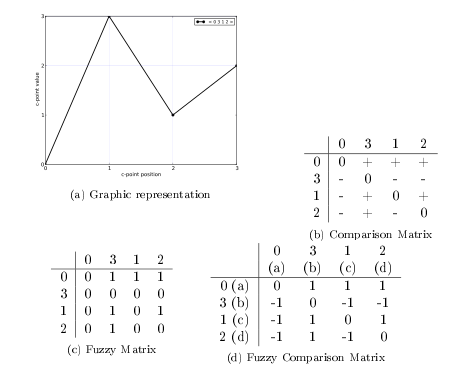
Figure 1: Contour and matrices of Cseg < 0 3 1 2 >
The Fuzzy Matrix uses fuzzy comparison. We can see the Fuzzy Matrix for < 0 3 1 2 > in table 1c.
The Fuzzy Comparison Matrix is based on the Fuzzy Matrix. The Cartesian positions of Fuzzy Comparison Matrix are the Fuzzy Comparison between opposite Cartesian positions of Fuzzy Matrix. For example, the Cartesian position ) , in table 1d is given by
, in table 1d is given by -\mu_{C^+}(b,a)) of Fuzzy Matrix, in table 1c. Thus, the position
of Fuzzy Matrix, in table 1c. Thus, the position .
2.2 Reduction operations
The reduction algorithms by Morris (1993) and Bor (2009) are two distinct algorithms that consider the change of direction as the most important points in a cseg. Each c-point is compared with its neighbors, and removed if is not the highest or lowest. While Morris’ algorithm removes and compares c-points globally, Bor’s compares them locally and they often yield different results (see table 1). A complete explanation about the algorithms or their differences is out of the scope of this paper, but is well documented in Bor (2009).
2.3 Similarity operations
We can use the Contour Similarity (CSIM) (Marvin 1988) and Fuzzy Similarity (Quinn 1997) operations to compare csegs with the same cardinality and the All Mutually Embedded Contour Segment (ACMEMB) (Marvin 1988) operation to compare csegs with different cardinality. CSIM and Fuzzy Similarity are based on matrix comparison, and ACMEMB is based on all embedded subsets of the compared csegs.
A matrix similarity is an average of the equal values of Cartesian positions in two matrices with the same cardinality. For instance, figure 2 has only one different Cartesian position between the two matrices. Since the matrix is symmetric, we compare only superior triangle. In this case the similarity value is 5/6, or 0.83.
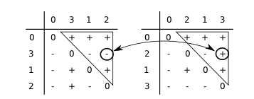
Figure 2: Matrix superior triangle positions comparison
The Comparison Similarity and Fuzzy Similarity differs only in the base matrix. The former uses Comparison Matrix, and the second, Fuzzy Comparison Matrix.
The operation All Mutually Embedded Contour Segment (ACMEMB) returns a numeric measure for similarity between two csegs of different or similar cardinality. The number of all csubsegs mutually embedded in both csegs is divided by the total of possible csubsegs in both csegs. For instance, < 0 3 1 2 4 >, and < 0 2 1 3 > have 37 possible csubsegs in common, and 32 mutually embedded csubsegs, therefore their ACMEMB is 0.86.
3 Music21
Music21 has many features such as advanced ways to analyze and transform music data and different types of visualization. In this section we’ll see how Music21 works in a brief example, however, a full tutorial is out of the scope of this paper. For more information see Cuthbert (2010), Ariza (2010) and its documentation at http://mit.edu/music21.
As a simple illustration, the following script calculates the five most common notes in Bach’s Chorale #1. The script takes advantage of both Music21’s and Python’s capabilities. Music21 takes care of parsing the humdrum file and returning a flat list with all notes from the four voices. Python’s class Counter automatically counts the number of elements in a list and returns a list of the five most common notes (using the method most_common):
music = music21.parse("001.krn")
notes = music.flat.notes
names = [note.name for note in notes]
count = Counter(names)
print count.most_common(5)
The result shows, unsurprisingly, that the notes G, D, B, C and A are the most common. One of the biggest advantages of using a general purpose language such as Python for music analysis is that one can abstract problems with functions and classes and easily re-use code. We can use the same script to count the most used notes in a different composition, by changing just one line of code:
music = music21.parse("bwv1048a.krn")
This will count the five most common notes in Bach’s Brandenburg Concerto No.3 in G major (first movement). The result, as expected, is similar to the Chorale; the most common notes are D, G, B, A, E.
4 The contour module
The contour module extends Music21 with contour processing capabilities. The following example shows a small script to return the two most common reduced contours in Bach’s Chorale #1 according to three algorithms; Morris Reduction (Morris 1993), Bor Reduction 35 (Bor 2009), and Bor Reduction 53 (Bor 2009).2
def split_phrases(part):
    nts = part.flat.notes.stripTies()
    pos = [x for x, n in enumerate(nts) if has_fmt(n)]
    return [nts[s+1:e+1] for s, e in zip([0]+pos, pos)]


def all_contours(music):
    contours = []
    for part in music.parts:
        for phrase in split_phrases(part):
            contours.append(Contour(phrase))
    return contours


def reduction(contour, fn):
    return tuple(apply_fn(contour, fn)[0])


music = music21.parse("001.krn")
for fn in ['reduction_morris',
           'reduction_morris',
           'reduction_bor_35',
           'reduction_bor_53']:
    red=[reduction(c, fn) for c in all_contours(music)]
    print fn, Counter(red).most_common(2)
The function split_phrases receives a Music21 Stream containing a voice and returns a list of phrases defined by fermatas. The function all_contours returns a flat list with all contours in every voice in a music Stream. Finally, the utility function reduction applies a reduction algorithm. Having defined these functions, the process to count the most common contour is the same as counting the most common notes. The most common contour in this Chorale is < 1 2 0 >, however the second most common is different for each algorithm. We can see the result for each algorithm in table 1.
| Cseg | First | Second |
|---|---|---|
| Morris | < 1 2 0 > | < 1 0 3 2 > |
| Bor 35 | < 1 2 0 > | < 0 2 0 1 > |
| Bor 53 | < 1 2 0 > | < 0 1 0 > |
In the following sections we investigate and compare some contour characteristics on all Bach’s 371 Chorales. In these examples “phrases” are voices segmented by fermata markings.
4.1 Highest c-points
A cseg can be more or less diversified than other with the same cardinality. For instance, < 0 1 2 3 > has more different c-points than < 0 1 0 1 >. We used the code in the following example to measure the voice with the most diversified phrase segments.
def higher_cpoints(phrs):
    dic = defaultdict(list)
    contour_group = group_phrases(phrs)
    for cseg, g_phrs in contour_group.items():
        for phr in g_phrs:
            dic[max(cseg)].append(phr)
    return dic


def higher_cpoints_count(phrs):
    pts = higher_cpoints(phrs)
    r = [(cp, len(phr_l)) for cp, phr_l in pts.items()]
    return sorted(r, key=lambda x: x[1], reverse=True)


def higher_cpoints_values_3_to_7(phrs):
    def aux(cpoints, cp_s, p_size):
        r = [cp for cp, s in cpoints if cp in cp_s]
        return sum(r) * 100.0 / p_size

    result = []
    for voice, phr in group_by_voice(phrs):
        cps = higher_cpoints_count(phr)
        p_size = len(phr)
        cp_size = [[3, 4, 5], [6, 7]]
        r = [aux(cps, cp_s, p_size) for cp_s in cp_size]
        result.append((voice, r))
    return result
We counted the percentage of phrases in which the highest c-point was either 3, 4, or 5 (group A) and 6 or 7 (group B). A voice has more more diversified csegs if it has a higher percentage of phrases in group B. We can see the result in table 2 and figure 3. The bass is the voice with the highest percentage of phrases in group B (43.04%), therefore, we can conclude that it’s the voice with the most diversified csegs in all of Bach’s Chorales. This result makes sense, since in a four-part chorale the lowest voice has more jumps while the other voices are more linear and melodic.
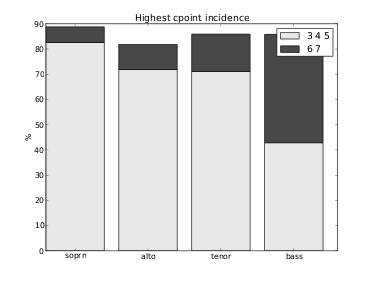
Figure 3: C-point size incidence in most common phrases
| Voice | Group A | Group B |
|---|---|---|
| Soprano | 82.64% | 06.15% |
| Alto | 71.88% | 09.93% |
| Tenor | 71.15% | 14.78% |
| Bass | 42.82% | 43.04% |
4.2 Common versus unique phrases
We can measure how diversified the voices are by comparing the amount of unique and repeated csegs. In the following script, we organized all phrases in each voice by their csegs and counted how many phrases have the same cseg3
seq = count_dic_items(group_phrases(phrs))
common_phrs = sort_descendent(seq)
most_common = sum([x[1] for x in common_phrs[:n]])
total = len(seq)
unique = 0
for [p, value] in common_phrs:
    if value == 1: unique += 1
return** perc(unique, total), perc(most_common, total)

def common_unique(phrs):
    r = []
    for voice, phr in group_by_voice(phrs):
        data = common_unique_aux(phr)
        r.append((voice, data))
    return r
Alto, tenor and bass have a balanced proportion between unique and repeated csegs, around 80%. However, the soprano has more repeated csegs than the other voices (see figure 4).
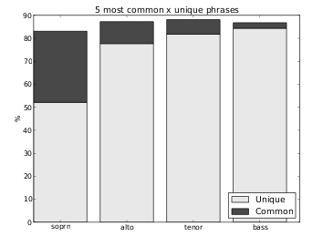
Figure 4: Common x unique phrases in all voices
4.3 Similarity in reduced phrases csegs
We checked the similarity among common phrases in all voices using Morris’ algorithm (Morris 1993). In the following script the function comparison_similarity returns a similarity index using Fuzzy or ACMEMB operations depending on the cseg’s cardinality (see section 2.3).
The function similarity_all_reduced returns similarity indices for all combinations of two elements and the number of times the reduced cseg occur.
Figure 5 shows the similarity indices for all compared csegs. For example, the reduced csegs < 1 0 > and < 1 2 0 > have a similarity index of 0.6 with 3179 csegs reduced to one of these forms (see the rightmost point in the figure). There isn’t an uniform distribution between the number of csegs with the same reduced form and their similarity index.
def comparison(data, total_number):
    (cseg1, phrs_n1), (cseg2, phrs_n2) = data
    sim = similarity.comparison_similarity(cseg1, cseg2)
    return [sim, phrs_n1 + phrs_n2]


def similarity_all_reduced(phrases):
    dic = reduction.morris_form_dict(phrases)
    seq = [[Contour(k), v] for k, v in dic.items()]
    total = len(dic.values())
    comb = itertools.combinations(seq, 2)
    y = sort_desc([comparison(c, total) for c in comb])
    sim = [] phrs
    n = []
    for s, p in y:
        sim.append(s)
        phrs_n.append(p)
    return phrs_n, sim
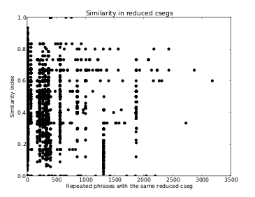
Figure 5: Similarity among all phrases reduced csegs
5 Conclusion
In this paper we presented the contour module for the Music21 toolkit and how it can be used for Contour Theory analysis. This is the only tool available for contour analysis today and we believe that it can help with the study and application of Contour Theory.
Using the module we could see that the bass is the voice with the most diversified contour segments and the soprano is the voice with more repeated contour segments in the 371 Bach Chorales. Naturally, this type of analysis can be applied for other group of compositions as well.
References
Ariza, Christopher. 2010. “Modeling Beats, Accents, Beams, and Time Signatures Hierarchically with Music21 Meter Objects”. In Proceedings of International Computer Music Conference.
Beard, R. D. 2003. Contour Modeling by Multiple Linear Regression of the Nineteen Piano Sonatas by Mozart. Phd dissertation, Florida State University.
Bor, Mustafa. 2009. Contour Reduction Algorithms: a Theory of Pitch and Duration Hierarchies for Post-tonal Music. Phd dissertation, University of British Columbia.
Clifford, Robert J. 1995. Contour as a Structural Element in Selected Pre-serial Works by Anton Webern. Phd dissertation, University of Wisconsin-Madison.
Cuthbert, Michael S. and Christopher Ariza. 2010. “Music21 A Toolkit for Computer-Aided Musicology and Symbolic Music Data”. In Proceedings of International Symposium on Music Information Retrieval.
Cuthbert, Michael S. and Christopher Ariza with Lisa Friedland. 2011. “Feature Extraction and Machine Learning on Symbolic Music using the music21 Toolkit”. In Proceedings of International Symposium on Music Information Retrieval.
Friedmann, Michael L. 1985. “A Methodology for the Discussion of Contour: Its Application to Schoenberg’s ‘Music’”. In Journal of Music Theory, 29(2): 223.
Levé, Florence and Richard Groult with Guillaume Arnaud, Cyril Séguin, Rémi Gaymay, and Mathieu Giraud. 2011. “Rhythm Extraction from Polyphony Symbolic Music”. In Proceedings of International Symposium on Music Information Retrieval.
Marvin, Elizabeth W. 1988. A Generalized Theory of Musical Contour: its Application to Melodic and Rhythmic Analysis of Non-tonal Music and its Perceptual and Pedagogical Implications. Phd dissertation, University of Rochester.
Morris, Robert D. 1987. Composition with Pitch-classes: A Theory of Compositional Design. New Haven: Yale University Press.
_____. “New Directions in the Theory and Analysis of Musical Contour”. 1993. Music Theory Spectrum 15(2): 205–228 (October).
Pérez, Fernando and Brian E. 2007. “Granger. IPython: a System for Interactive Scientific Computing”. Comput. Sci. Eng., 9(3): 21–29 (May).
Polansky, Larry and Richard Bassein. 1992. “Possible and Impossible Melody: Some Formal Aspects of Contour”. Journal of Music Theory 36(2): 259.
Quinn, Ian. 1997. “Fuzzy Extensions to the Theory of Contour”. Music Theory Spectrum 19(2): 232–263.
Schultz, Rob D. 2008. “Melodic Contour and Nonretrogradable Structure in the Birdsong of Olivier Messiaen”. Music Theory Spectrum 30(1): 89–137 (April).
Zadeh, Lofti A. 1965. “Fuzzy Sets”. Information and Control 8(3): 338–353.
Notes:
1 In order to make the code fit in the two-column layout we used shorter names than we’d normally use such as has_fmt instead of has_fermata and nts instead of notes.
2We removed the duplicate sopranos since Bach harmonized 42 melodies twice.